BEFORE YOU BEGIN... 
You first need the data you wish to plot in a form acceptable for tikz. I find that table data with headers is easiest (file type .dat). This can be easily generated using MATLAB.

Some tips: 

1. ​You likely have MORE data than you actually need to make a nice plot. In order to speed up compilation time, reduce your data as much as possible while still getting a smooth curve. (I found about 200 points is sufficient for a standard sized figure.)
   
2. Organizing your data such that each file contains a different set of data, but the same header labels will make generating plots much more automated.

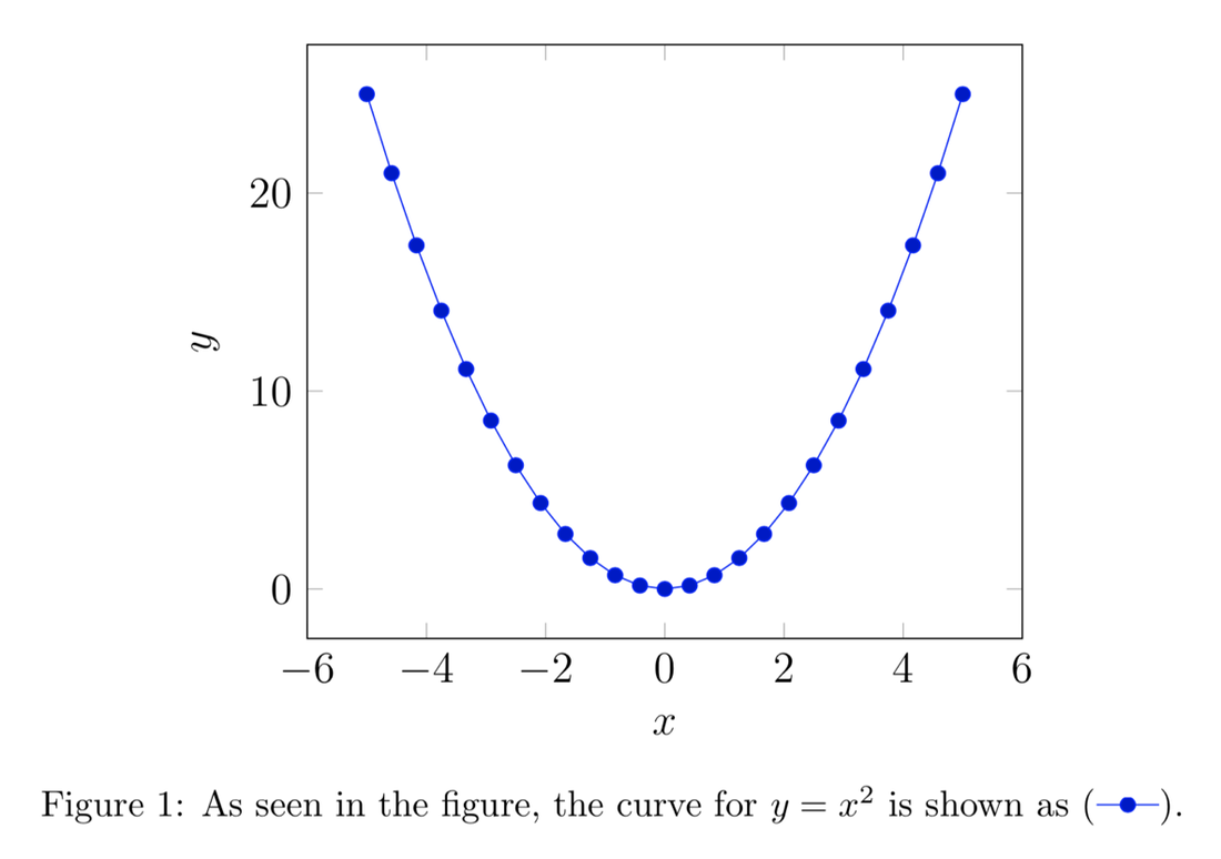
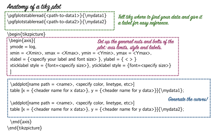Next, you're going to want to add a few things to the preamble of your file.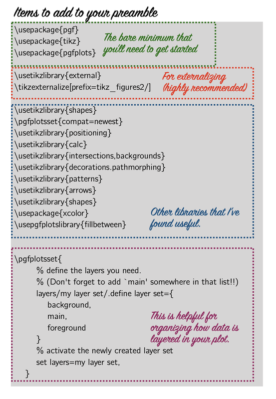 

Now, let's look at a fairly simple example. The tex code is on the left, and the resulting plot is on the right.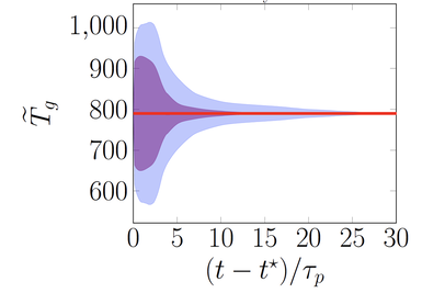 

\pgfplotstableread{tikz/Data_CIT_0D.dat}{\zero}
\pgfplotstableread{tikz/Data_CIT_2D.dat}{\two}
\pgfplotstableread{tikz/Data_CIT_3D.dat}{\three}
\begin{tikzpicture}
   \begin{axis}[
     xmin=0, xmax=30, 
     xlabel={\LARGE $(t-t^\star)/\tau_p$}, ylabel={\LARGE$ \widetilde{T}_g $},
     yticklabel style = {font=\LARGE},  xticklabel style = {font=\LARGE}, 
  ]

    \addplot[name path = A, black, solid, line width = 2pt] 
     table [x={t}, y = {T_mean}] {\two}; \label{2D}

    \addplot[name path = B, blue, opacity = 0.25, line width = 0pt] 
     table [x={t}, y = {T_up}] {\two};

    \addplot[name path = C, blue, opacity = 0.25, line width = 0pt] 
     table [x={t}, y = {T_down}] {\two};

    \addplot[blue, opacity =0.25] fill between[of=B and C]; 

    \addplot[name path = A, black, solid, line width = 2pt] 
     table [x={t}, y = {T_mean}] {\three};

    \addplot[name path = B, violet, opacity =.50, solid, line width = 0pt] 
     table [x={t}, y = {T_up}] {\three};

    \addplot[name path = C, violet, opacity = 0.50, solid, line width = 0pt] 
     table [x={t}, y = {T_down}] {\three}; 

    \addplot[violet, opacity = 0.5] fill between[of=B and C]; 

    \addplot[black, solid, line width = 2pt] 
    table [x={t}, y = {T_mean}] {\zero};
​
      \end{axis}
\end{tikzpicture}

EXTERNALIZING TIKZ.... 

If you plan to generate a large number of figures using tikz (especially if these files contain a lot of data), you’ll want to externalize tikz so that your main LaTeX file doesn’t have to recompile all of the figures every time you compile the main document (this can take a long time and LaTeX can also run out of the memory required to do it at all, even if you don’t mind the wait). Fortunately, this is pretty easy! 

1. First you will need to set up your compiler to handle the externalization. For TeXShop, this is done by going to Preferences>Engine, then in the field for “LaTeX”, you need to add “-- shell-escape” to the end. It should read: pdflatex --file-line-error --synctex=1 —shell-escape.
   
2. Then, you will need to create a folder where you want to send the tikz figures (this can be the same folder where you’re keep other figures for the main document, or it can be different). 
   
3. Next, you want to open a separate LaTeX file, solely for generating the tikz figures. Keep in mind you may want to borrow a good deal of the preamble from your main LaTeX file so that you have the math symbols or colors you defined there. Also make sure that you specify \usetikzlibrary{external} and \tikzexternalize[prefix = <path to that folder you just created>] 
   
4. Now, you can start coding your tikz figures!

EASY REFERENCE OF SYMBOLS IN CAPTIONS

Tikz makes it seamless to integrate a legend or refer to symbols/lines in the figure within a caption. All that is required to do this is to label each of your plots using \label{<name this plot>} and can then use the command \ref{<name the plot>} in the caption or elsewhere in the text.

If you have externalized your tikz figures, you'll need to handle caption legends a bit differently. In the preamble to your main document you will need to define a tikz picture for your legend. An example of this is for a blue, dashed line is:

 \newcommand{\ModelTp}{\raisebox{6pt}{\tikz{\draw[blue,dashed,line width=3pt](0,0) -- (16mm,0);}}}

Then, you'll need to reference it in the caption as:

​\protect \ModelTp 

Here, the '\protect' is needed to allow a tikz picture to show up in the caption text. 

Learning LaTeX can be a daunting task, especially when you're teaching yourself and stuck consulting stack exchange for hours on end. To spare others some of those early growing pains, I've created a quick start guide, as well as a template. The template includes the main pieces that I have used time and time again in drafting papers and reports.  

1. You'll need to install a tex previewer (it essentially is an editor in which you can code up your document, compile it and view the resulting pdf). I like TeXShop, but there are other options as well. 
2. Some basic document structure: A tex file (the code that generates your document) has two main parts: the preamble (which is where you include packages, define shortcuts, set colors, set the document type and style, etc) and the main document, where the content of your document lives (this is all sandwiched between \begin{document} and \end{document}). You will also likely have a bibliography file as well (extension .bib), that will be used to generate your bibliography and organize references (there will be a separate post on this topic). 
3. The building blocks:
   1. Text: This is the most straight forward portion of the document. As long as you're between \begin{document} and \end{document}, you can enter text just like a standard word processor. It's worth noting that you can divide up your text into sections with \section{Name of Section}. This will automatically number/letter (depending on the style and type of document chosen in the preamble) the text of your section name and give it a unique font/size compared with the rest of the main body of text. 
   2. Tables: Tables come up quite a lot for me, so I've included a simple table as well as a more complex, nicer looking one in the template. The basic structure for a simple table is shown below. The 'table' environment (\begin{table} \end{table}) will allow you to label and caption the table, and the 'tabular' environment  (\begin{tabular} \end{tabular}) is what actually generates the structure of the table. Next to \begin{tabular} is where you can define the number of columns, as well as their alignment (c = center, l = left, r = right). The vertical bar key can be used here to insert vertical lines between columns. You can also add additional (or less) space between columns here as well. Finally, inside the tabular environment, rows of your table are separated with '//' (this is a line break command) and columns are delineated with '&'. Always make sure that you have the same number of items in each row (i.e. same number of columns) as you do in your definition. Within the table, horizontal lines can be added using '\hline' (note: this is not the only way to achieve horizontal lines). 

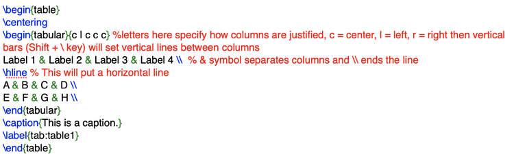3. Figures: You will undoubtedly need to add images/plots/figures to your document and this is pretty straight forward. Similarly to the table example, you first generate the figure environment (\begin{figure} \end{figure}) which will label your figure and give it a caption (if you choose). Inside of this environment, you include an image using \includegraphics[<specify scale, height or width of the image here>]{<specify the path to the file relative to the location of your .tex file>}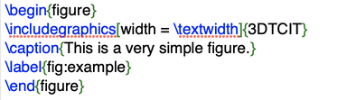   

4. Equations: For me, writing equations is the biggest selling point for LaTeX. Once you get used to coding up equations, this method is so much quicker than any other equation editor and looks orders of magnitude nicer too. The two main equation environments that I use are the 'equation' environment (\begin{equation} \end{equation}) and the align environment (\begin{align} \end{align}). The main difference between these two is that the align environment allows you to (as the name suggests) align lines of equations, using the '&' key. This is handy for making your equations look cleaner and more organized, or to display an equation that is too long for a single line. Both these environments will by default number your equations. If you do not want a number, you can either include \nonumber at the end of the equation, or, you can use the equation* or align* environments. You can also enter into 'math' mode inline in your document using $ <put your equation code here> $. Using $$ $$ will cause a line break and display like \begin{equation*} \end{equation*}.  

To serve as a launching off point, here is a template with all the main building blocks that I tend to use regularly. I hope you find it to be helpful! 

When starting out with LaTeX, you'll undoubtedly ask yourself, 'But isn't [insert text editor you usually use] so much quicker/easier/etc.?' Maybe it is right now, but with practice, typesetting with LaTeX is quicker and looks more polished (especially when creating documents with lots of equations). In fact, once you get the hang of coding in LaTeX, you'll realize how time-consuming the equation editor in ppt and word really was and how much more streamlined having control over all aspects of the typesetting is.